Dictionary Learning for cross-modality integration
Compiled: October 31, 2023
Source:vignettes/seurat5_integration_bridge.Rmd
seurat5_integration_bridge.RmdIn the same way that read mapping tools have transformed genome sequence analysis, the ability to map new datasets to established references represents an exciting opportunity for the field of single-cell genomics. Along with others in the community, we have developed tools to map and interpret query datasets, and have also constructed a set of scRNA-seq datasets for diverse mammalian tissues.
A key challenge is to extend this reference mapping framework to technologies that do not measure gene expression, even if the underlying reference is based on scRNA-seq. In Hao et al, Nat Biotechnol 2023, we introduce ‘bridge integration’, which enables the mapping of complementary technologies (like scATAC-seq, scDNAme, CyTOF), onto scRNA-seq references, using a ‘multi-omic’ dataset as a molecular bridge. In this vignette, we demonstrate how to map an scATAC-seq dataset of human PBMC, onto our previously constructed PBMC reference. We use a publicly available 10x multiome dataset, which simultaneously measures gene expression and chromatin accessibility in the same cell, as a bridge dataset.
In this vignette we demonstrate:
- Loading in and pre-processing the scATAC-seq, multiome, and scRNA-seq reference datasets
- Mapping the scATAC-seq dataset via bridge integration
- Exploring and assessing the resulting annotations
Azimuth ATAC for Bridge Integration
Users can now automatically run bridge integration for PBMC and Bone Marrow scATAC-seq queries with the newly released Azimuth ATAC workflow on the Azimuth website or in R. For more details on running locally in R, see the section on ATAC data in this vignette.
Load the bridge, query, and reference datasets
We start by loading a 10x multiome dataset, consisting of ~12,000 PBMC from a healthy donor. The dataset measures RNA-seq and ATAC-seq in the same cell, and is available for download from 10x Genomics here. We follow the loading instructions from the Signac package vignettes. Note that when using Signac, please make sure you are using the latest version of Bioconductor, as users have reported errors when using older BioC versions.
Load and setup the 10x multiome object
# the 10x hdf5 file contains both data types.
inputdata.10x <- Read10X_h5("/brahms/hartmana/vignette_data/pbmc_cellranger_arc_2/pbmc_granulocyte_sorted_10k_filtered_feature_bc_matrix.h5")
# extract RNA and ATAC data
rna_counts <- inputdata.10x$`Gene Expression`
atac_counts <- inputdata.10x$Peaks
# Create Seurat object
obj.multi <- CreateSeuratObject(counts = rna_counts)
# Get % of mitochondrial genes
obj.multi[["percent.mt"]] <- PercentageFeatureSet(obj.multi, pattern = "^MT-")

# add the ATAC-seq assay
grange.counts <- StringToGRanges(rownames(atac_counts), sep = c(":", "-"))
grange.use <- seqnames(grange.counts) %in% standardChromosomes(grange.counts)
atac_counts <- atac_counts[as.vector(grange.use), ]
# Get gene annotations
annotations <- GetGRangesFromEnsDb(ensdb = EnsDb.Hsapiens.v86)
# Change style to UCSC
seqlevelsStyle(annotations) <- 'UCSC'
genome(annotations) <- "hg38"
# File with ATAC per fragment information file
frag.file <- "/brahms/hartmana/vignette_data/pbmc_cellranger_arc_2/pbmc_granulocyte_sorted_10k_atac_fragments.tsv.gz"
# Add in ATAC-seq data as ChromatinAssay object
chrom_assay <- CreateChromatinAssay(
  counts = atac_counts,
  sep = c(":", "-"),
  genome = 'hg38',
  fragments = frag.file,
  min.cells = 10,
  annotation = annotations
)
# Add the ATAC assay to the multiome object
obj.multi[["ATAC"]] <- chrom_assay
# Filter ATAC data based on QC metrics
obj.multi <- subset(
  x = obj.multi,
  subset = nCount_ATAC < 7e4 &
    nCount_ATAC > 5e3 &
    nCount_RNA < 25000 &
    nCount_RNA > 1000 &
    percent.mt < 20
)
The scATAC-seq query dataset represents ~10,000 PBMC from a healthy donor, and is available for download here. We load in the peak/cell matrix, store the path to the fragments file, and add gene annotations to the object, following the steps as with the ATAC data in the multiome experiment.
We note that it is important to quantify the same set of genomic features in the query dataset as are quantified in the multi-omic bridge. We therefore requantify the set of scATAC-seq peaks using the FeatureMatrix command. This is also described in the Signac vignettes and shown below.
Load and setup the 10x scATAC-seq query
# Load ATAC dataset
atac_pbmc_data <- Read10X_h5(filename = "/brahms/hartmana/vignette_data/10k_PBMC_ATAC_nextgem_Chromium_X_filtered_peak_bc_matrix.h5")
fragpath <- "/brahms/hartmana/vignette_data/10k_PBMC_ATAC_nextgem_Chromium_X_fragments.tsv.gz"
# Get gene annotations
annotation <- GetGRangesFromEnsDb(ensdb = EnsDb.Hsapiens.v86)
# Change to UCSC style
seqlevelsStyle(annotation) <- 'UCSC'
# Create ChromatinAssay for ATAC data
atac_pbmc_assay <- CreateChromatinAssay(
  counts = atac_pbmc_data,
  sep = c(":", "-"),
  fragments = fragpath,
  annotation = annotation
)
# Requantify query ATAC to have same features as multiome ATAC dataset
requant_multiome_ATAC <- FeatureMatrix(
  fragments = Fragments(atac_pbmc_assay),
  features = granges(obj.multi[['ATAC']]),
  cells = Cells(atac_pbmc_assay)
)
# Create assay with requantified ATAC data
ATAC_assay <- CreateChromatinAssay(
  counts = requant_multiome_ATAC,
  fragments = fragpath,
  annotation = annotation
)
# Create Seurat sbject
obj.atac  <- CreateSeuratObject(counts = ATAC_assay,assay = 'ATAC')
obj.atac[['peak.orig']] <- atac_pbmc_assay
obj.atac <- subset(obj.atac, subset = nCount_ATAC < 7e4 & nCount_ATAC > 2000)
We load the reference (download here) from our recent paper. This reference is stored as an h5Seurat file, a format that enables on-disk storage of multimodal Seurat objects (more details on h5Seurat and SeuratDisk can be found here).
obj.rna <- readRDS("/brahms/haoy/seurat4_pbmc/pbmc_multimodal_2023.rds")What if I want to use my own reference dataset?
As an alternative to using a pre-built reference, you can also use your own reference. To demonstrate, you can download a scRNA-seq dataset of 23,837 human PBMC here, which we have already annotated.
obj.rna = readRDS("/path/to/reference.rds")
obj.rna = SCTransform(object = obj.rna) %>%
  RunPCA() %>%
  RunUMAP(dims = 1:50, return.model = TRUE)
When using your own reference, set reference.reduction = "pca" in the PrepareBridgeReference function.
Preprocessing/normalization for all datasets
Prior to performing bridge integration, we normalize and pre-process each of the datasets (note that the reference has already been normalized). We normalize gene expression data using sctransform, and ATAC data using TF-IDF.
# normalize multiome RNA
DefaultAssay(obj.multi) <- "RNA"
obj.multi <- SCTransform(obj.multi, verbose = FALSE)
# normalize multiome ATAC
DefaultAssay(obj.multi) <- "ATAC"
obj.multi <- RunTFIDF(obj.multi)
obj.multi <- FindTopFeatures(obj.multi, min.cutoff = "q0")
# normalize query
obj.atac <- RunTFIDF(obj.atac)
Map scATAC-seq dataset using bridge integration
Now that we have the reference, query, and bridge datasets set up, we can begin integration. The bridge dataset enables translation between the scRNA-seq reference and the scATAC-seq query, effectively augmenting the reference so that it can map a new data type. We call this an extended reference, and first set it up. Note that you can save the results of this function and map multiple scATAC-seq datasets without having to rerun.
First, we drop the first dimension of the ATAC reduction.
dims.atac <- 2:50
dims.rna <- 1:50
DefaultAssay(obj.multi) <-  "RNA"
DefaultAssay(obj.rna) <- "SCT"
obj.rna.ext <- PrepareBridgeReference(
  reference = obj.rna, bridge = obj.multi,
  reference.reduction = "spca", reference.dims = dims.rna,
  normalization.method = "SCT")
Now, we can directly find anchors between the extended reference and query objects. We use the FindBridgeTransferAnchors function, which translates the query dataset using the same dictionary as was used to translate the reference, and then identifies anchors in this space. The function is meant to mimic our FindTransferAnchors function, but to identify correspondences across modalities.
bridge.anchor <- FindBridgeTransferAnchors(
  extended.reference = obj.rna.ext, query = obj.atac,
  reduction = "lsiproject", dims = dims.atac)
Once we have identified anchors, we can map the query dataset onto the reference. The MapQuery function is the same as we have previously introduced for reference mapping . It transfers cell annotations from the reference dataset, and also visualizes the query dataset on a previously computed UMAP embedding. Since our reference dataset contains cell type annotations at three levels of resolution (l1 - l3), we can transfer each level to the query dataset.
obj.atac <- MapQuery(
  anchorset = bridge.anchor, reference = obj.rna.ext,
  query = obj.atac,
  refdata = list(
    l1 = "celltype.l1",
    l2 = "celltype.l2",
    l3 = "celltype.l3"),
  reduction.model = "wnn.umap")
Now we can visualize the results, plotting the scATAC-seq cells based on their predicted annotations, on the reference UMAP embedding. You can see that each scATAC-seq cell has been assigned a cell name based on the scRNA-seq defined cell ontology.
DimPlot(
  obj.atac, group.by = "predicted.l2",
  reduction = "ref.umap", label = TRUE
) + ggtitle("ATAC") + NoLegend()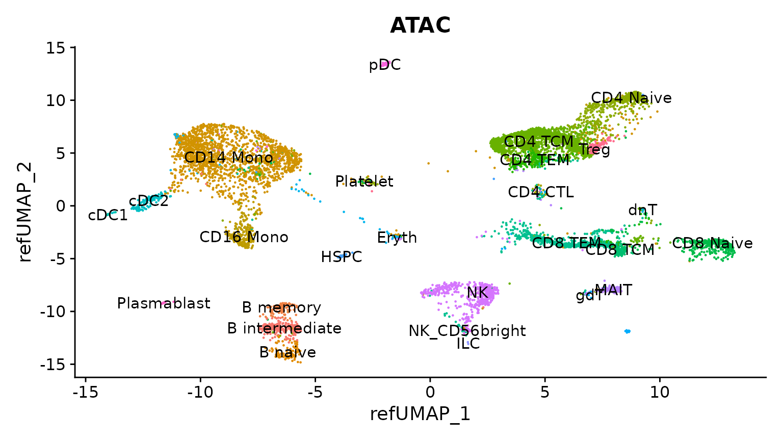
Assessing the mapping
To assess the mapping and cell type predictions, we will first see if the predicted cell type labels are concordant with an unsupervised analysis of the scATAC-seq dataset. We follow the standard unsupervised processing workflow for scATAC-seq data:
obj.atac <- FindTopFeatures(obj.atac, min.cutoff = "q0")
obj.atac <- RunSVD(obj.atac)
obj.atac <- RunUMAP(obj.atac, reduction = "lsi", dims = 2:50)
Now, we visualize the predicted cluster labels on the unsupervised UMAP emebdding. We can see that predicted cluster labels (from the scRNA-seq reference) are concordant with the structure of the scATAC-seq data. However, there are some cell types (i.e. Treg), that do not appear to separate in unsupervised analysis. These may be prediction errors, or cases where the reference mapping provides additional resolution.
DimPlot(obj.atac, group.by = "predicted.l2", reduction = "umap", label = FALSE)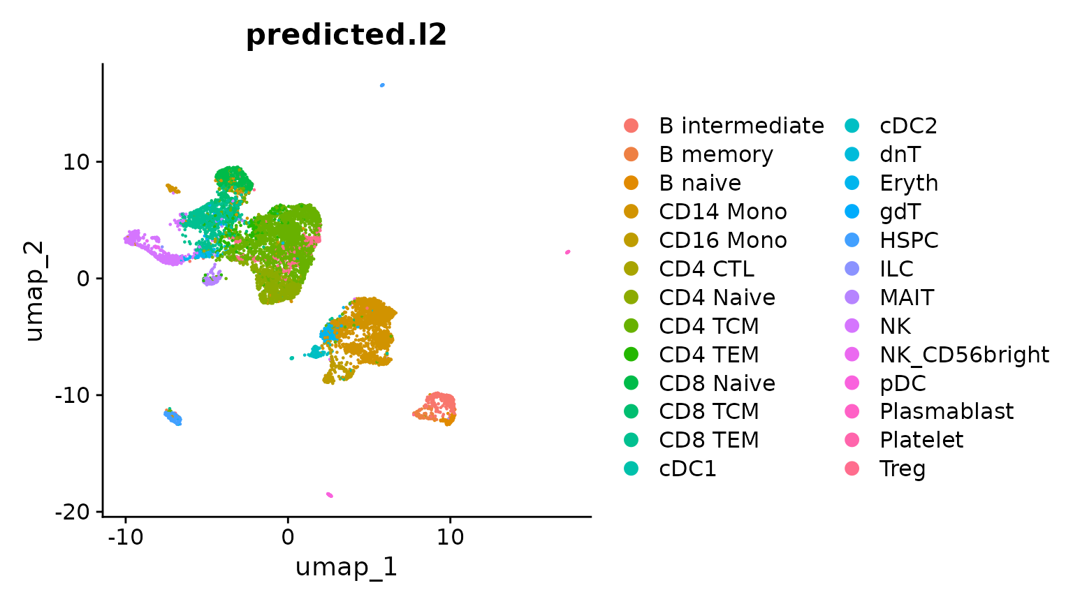
Lastly, we validate the predicted cell types for the scATAC-seq data by examining their chromatin accessibility profiles at canonical loci. We use the CoveragePlot function to visualize accessibility patterns at the CD8A, FOXP3, and RORC, after grouping cells by their predicted labels. We see expected patterns in each case. For example, the PAX5 locus exhibits peaks that are accessible exclusively in B cells, and the CD8A locus shows the same in CD8 T cell subsets. Similarly, the accessibility of FOXP3, a canonical marker of regulatory T cells (Tregs), in predicted Tregs provides strong support for the accuracy of our prediction.
CoveragePlot(
  obj.atac, region  = "PAX5", group.by = "predicted.l1",
  idents = c("B", "CD4 T", "Mono", "NK"), window = 200,
  extend.upstream = -150000)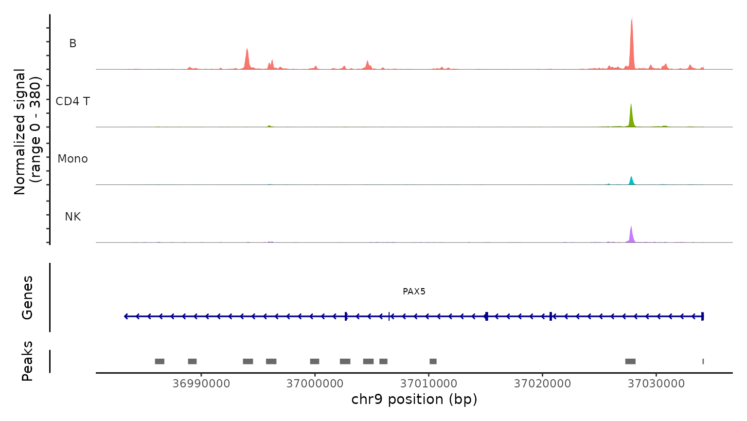
CoveragePlot(
  obj.atac, region = "CD8A", group.by = "predicted.l2",
  idents = c("CD8 Naive", "CD4 Naive", "CD4 TCM", "CD8 TCM"),
  extend.downstream = 5000, extend.upstream = 5000)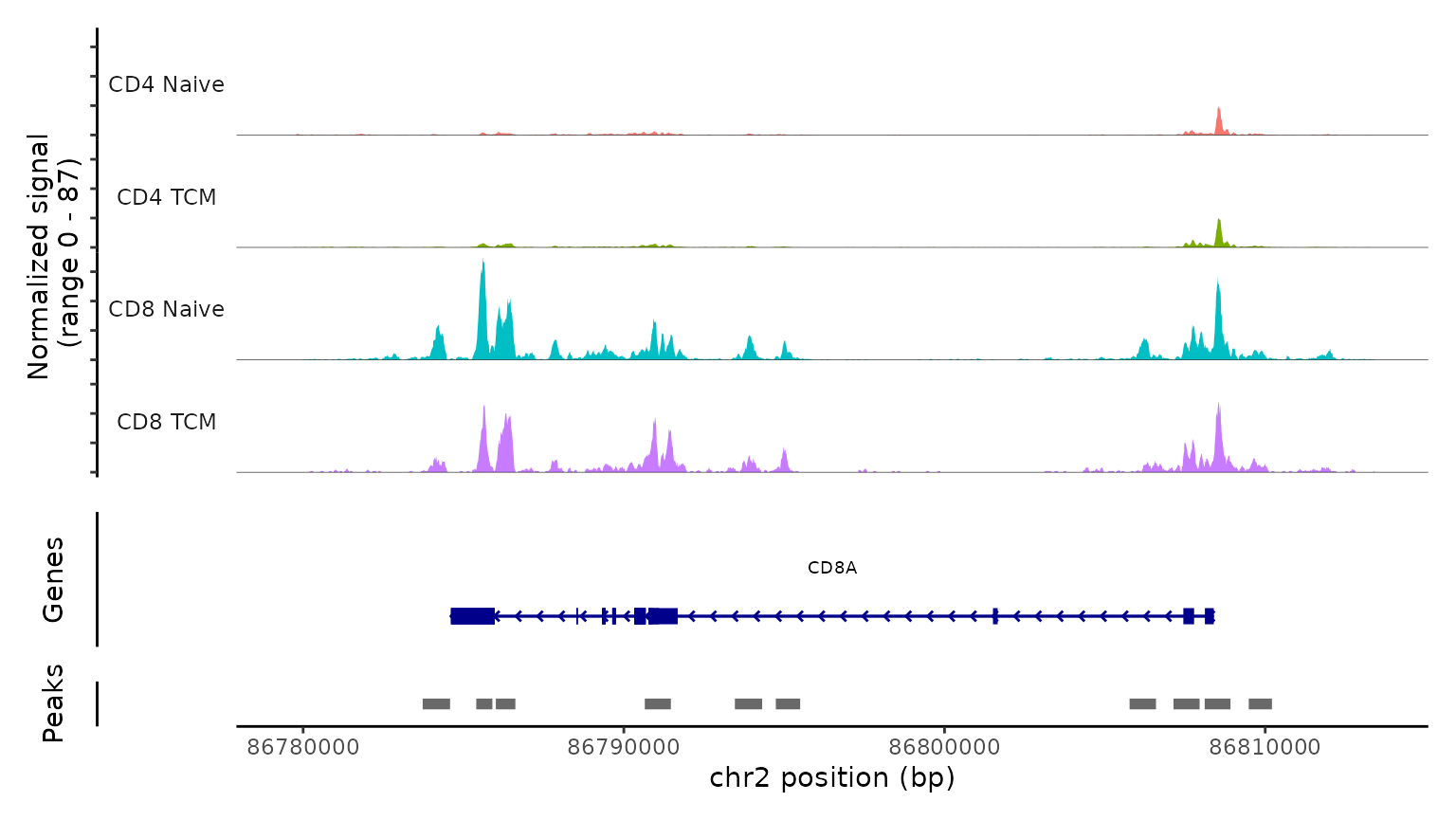
CoveragePlot(
  obj.atac, region = "FOXP3", group.by = "predicted.l2",
  idents = c( "CD4 Naive", "CD4 TCM", "CD4 TEM", "Treg"),
  extend.downstream = 0, extend.upstream = 0)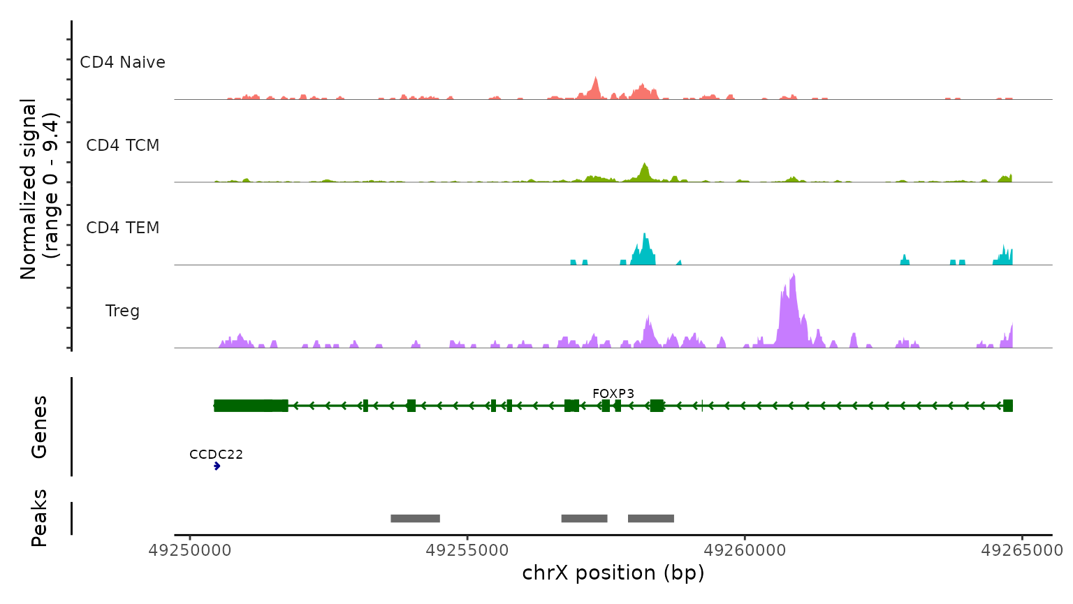
CoveragePlot(
  obj.atac, region = "RORC", group.by = "predicted.l2",
  idents = c("CD8 Naive", "CD8 TEM", "CD8 TCM", "MAIT"),
  extend.downstream = 5000, extend.upstream = 5000)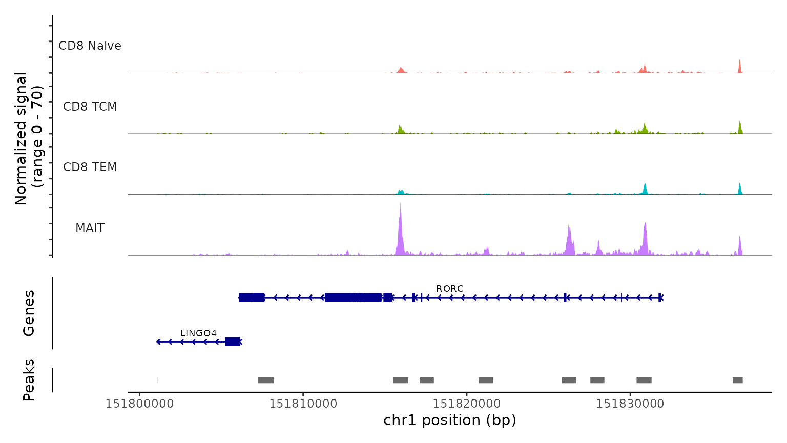
Session Info
## R version 4.2.2 Patched (2022-11-10 r83330)
## Platform: x86_64-pc-linux-gnu (64-bit)
## Running under: Ubuntu 20.04.6 LTS
##
## Matrix products: default
## BLAS:   /usr/lib/x86_64-linux-gnu/blas/libblas.so.3.9.0
## LAPACK: /usr/lib/x86_64-linux-gnu/lapack/liblapack.so.3.9.0
##
## locale:
##  [1] LC_CTYPE=en_US.UTF-8       LC_NUMERIC=C
##  [3] LC_TIME=en_US.UTF-8        LC_COLLATE=en_US.UTF-8
##  [5] LC_MONETARY=en_US.UTF-8    LC_MESSAGES=en_US.UTF-8
##  [7] LC_PAPER=en_US.UTF-8       LC_NAME=C
##  [9] LC_ADDRESS=C               LC_TELEPHONE=C
## [11] LC_MEASUREMENT=en_US.UTF-8 LC_IDENTIFICATION=C
##
## attached base packages:
## [1] stats4    stats     graphics  grDevices utils     datasets  methods
## [8] base
##
## other attached packages:
##  [1] ggplot2_3.4.4             dplyr_1.1.3
##  [3] EnsDb.Hsapiens.v86_2.99.0 ensembldb_2.22.0
##  [5] AnnotationFilter_1.22.0   GenomicFeatures_1.50.4
##  [7] AnnotationDbi_1.60.2      Biobase_2.58.0
##  [9] GenomicRanges_1.50.2      GenomeInfoDb_1.34.9
## [11] IRanges_2.32.0            S4Vectors_0.36.2
## [13] BiocGenerics_0.44.0       Signac_1.12.9000
## [15] Seurat_5.0.0              SeuratObject_5.0.0
## [17] sp_2.1-1
##
## loaded via a namespace (and not attached):
##   [1] rappdirs_0.3.3              rtracklayer_1.58.0
##   [3] scattermore_1.2             R.methodsS3_1.8.2
##   [5] ragg_1.2.5                  tidyr_1.3.0
##   [7] bit64_4.0.5                 knitr_1.45
##   [9] irlba_2.3.5.1               DelayedArray_0.24.0
##  [11] R.utils_2.12.2              styler_1.10.2
##  [13] data.table_1.14.8           rpart_4.1.19
##  [15] KEGGREST_1.38.0             RCurl_1.98-1.12
##  [17] generics_0.1.3              cowplot_1.1.1
##  [19] RSQLite_2.3.1               RANN_2.6.1
##  [21] future_1.33.0               bit_4.0.5
##  [23] spatstat.data_3.0-3         xml2_1.3.5
##  [25] httpuv_1.6.12               SummarizedExperiment_1.28.0
##  [27] xfun_0.40                   hms_1.1.3
##  [29] jquerylib_0.1.4             evaluate_0.22
##  [31] promises_1.2.1              fansi_1.0.5
##  [33] restfulr_0.0.15             progress_1.2.2
##  [35] dbplyr_2.3.4                igraph_1.5.1
##  [37] DBI_1.1.3                   htmlwidgets_1.6.2
##  [39] spatstat.geom_3.2-7         purrr_1.0.2
##  [41] ellipsis_0.3.2              RSpectra_0.16-1
##  [43] backports_1.4.1             biomaRt_2.54.1
##  [45] deldir_1.0-9                sparseMatrixStats_1.10.0
##  [47] MatrixGenerics_1.10.0       vctrs_0.6.4
##  [49] ROCR_1.0-11                 abind_1.4-5
##  [51] cachem_1.0.8                withr_2.5.2
##  [53] BSgenome_1.66.3             progressr_0.14.0
##  [55] checkmate_2.2.0             sctransform_0.4.1
##  [57] GenomicAlignments_1.34.1    prettyunits_1.1.1
##  [59] goftest_1.2-3               cluster_2.1.4
##  [61] dotCall64_1.1-0             lazyeval_0.2.2
##  [63] crayon_1.5.2                hdf5r_1.3.8
##  [65] spatstat.explore_3.2-5      pkgconfig_2.0.3
##  [67] labeling_0.4.3              nlme_3.1-162
##  [69] ProtGenerics_1.30.0         nnet_7.3-18
##  [71] rlang_1.1.1                 globals_0.16.2
##  [73] lifecycle_1.0.3             miniUI_0.1.1.1
##  [75] filelock_1.0.2              fastDummies_1.7.3
##  [77] BiocFileCache_2.6.1         dichromat_2.0-0.1
##  [79] rprojroot_2.0.3             polyclip_1.10-6
##  [81] RcppHNSW_0.5.0              matrixStats_1.0.0
##  [83] lmtest_0.9-40               Matrix_1.6-1.1
##  [85] zoo_1.8-12                  base64enc_0.1-3
##  [87] ggridges_0.5.4              png_0.1-8
##  [89] viridisLite_0.4.2           rjson_0.2.21
##  [91] bitops_1.0-7                R.oo_1.25.0
##  [93] KernSmooth_2.23-22          spam_2.10-0
##  [95] Biostrings_2.66.0           blob_1.2.4
##  [97] DelayedMatrixStats_1.20.0   stringr_1.5.0
##  [99] parallelly_1.36.0           spatstat.random_3.2-1
## [101] R.cache_0.16.0              scales_1.2.1
## [103] memoise_2.0.1               magrittr_2.0.3
## [105] plyr_1.8.9                  ica_1.0-3
## [107] zlibbioc_1.44.0             compiler_4.2.2
## [109] BiocIO_1.8.0                RColorBrewer_1.1-3
## [111] fitdistrplus_1.1-11         Rsamtools_2.14.0
## [113] cli_3.6.1                   XVector_0.38.0
## [115] listenv_0.9.0               patchwork_1.1.3
## [117] pbapply_1.7-2               htmlTable_2.4.1
## [119] Formula_1.2-5               MASS_7.3-58.2
## [121] tidyselect_1.2.0            stringi_1.7.12
## [123] textshaping_0.3.6           glmGamPoi_1.10.2
## [125] highr_0.10                  yaml_2.3.7
## [127] ggrepel_0.9.4               grid_4.2.2
## [129] sass_0.4.7                  VariantAnnotation_1.44.1
## [131] fastmatch_1.1-4             tools_4.2.2
## [133] future.apply_1.11.0         parallel_4.2.2
## [135] rstudioapi_0.14             foreign_0.8-84
## [137] gridExtra_2.3               farver_2.1.1
## [139] Rtsne_0.16                  digest_0.6.33
## [141] shiny_1.7.5.1               Rcpp_1.0.11
## [143] later_1.3.1                 RcppAnnoy_0.0.21
## [145] httr_1.4.7                  biovizBase_1.46.0
## [147] colorspace_2.1-0            XML_3.99-0.14
## [149] fs_1.6.3                    tensor_1.5
## [151] reticulate_1.34.0           splines_4.2.2
## [153] uwot_0.1.16                 RcppRoll_0.3.0
## [155] spatstat.utils_3.0-4        pkgdown_2.0.7
## [157] plotly_4.10.3               systemfonts_1.0.4
## [159] xtable_1.8-4                jsonlite_1.8.7
## [161] R6_2.5.1                    Hmisc_5.1-1
## [163] pillar_1.9.0                htmltools_0.5.6.1
## [165] mime_0.12                   glue_1.6.2
## [167] fastmap_1.1.1               BiocParallel_1.32.6
## [169] codetools_0.2-19            utf8_1.2.4
## [171] lattice_0.21-9              bslib_0.5.1
## [173] spatstat.sparse_3.0-3       tibble_3.2.1
## [175] curl_5.1.0                  leiden_0.4.3
## [177] survival_3.5-7              rmarkdown_2.25
## [179] desc_1.4.2                  munsell_0.5.0
## [181] GenomeInfoDbData_1.2.9      reshape2_1.4.4
## [183] gtable_0.3.4